SimpleLoader()
Loads REIXS Data vs Point Number
Class Information
Python
## PLOTING 1-D SIMPLE DATA ##
Simple = SimpleLoader()
## LOADING/ADDING/SUBSTRACTING 1-D/REDUCED DATA FROM A FILE ##
## Loads 1-D/Reduced scans data from HDF5 file
Simple.load(config,'filename', 'y_stream', *args, **kwargs)
## *args = comma seperated list of scans to be plotted
## Loads and sums 1-D/Reduced scans data from HDF5 file
Simple.add(config,'filename', 'y_stream', *args, **kwargs)
## *args = comma seperated list of scans to be plotted or added and then plotted
## Loads and subtratcs 1-D/Reduced scans data from HDF5 file
Simple.subtract(config,'filename', 'y_stream', *args, **kwargs)
## *args = s1, p1 -> The data from p1 is subtracted from s1
## *args = [s1, ..., sn], [p1, ..., pn] -> The sum of p1..pn is subtracted from the sum of s1...sn
## Loads and subtract scan from all previously loaded scans
Simple.background(config,'filename', 'y_stream', *args, **kwargs)
## *args = s1 -> The scan to be subtracted from all previous load/add/subtract actions
## *args = [s1, ..., sn] -> The sum of scans s1..sn to be subtracted from all load/add/subtract
## REQUIRED VARIABLES ##
## config = RIXS -> RIXS Endstation
## config = RSXS -> RSXS Endstation
## filename = hdf5 filename -> extenstion not required
## y_stream -> y-axis values, any mne or list from documentation
## NOTE: Simple math allowed with xes_stream with contstants and variables, i.e. +, -, /, *
## NOTES ON Y STREAMS ##
## The dimension of the y_stream needs to be 1
## The axis reduction for 2-D data types is y_stream[min:max] reducing dimension to 1
## The axis reduction for 3-D data types is y_stream[{min1:max1}, {min2:max2}]
## **kwargs ##
## norm = True -> Scales the data such that its range is 0 to 1.
## twin_y = True -> Adds these plots to a secondary scale
## yoffset = [(S1,P1),...,(SN,PN)] -> Adjusts y-axis scale to map SN to PN
## ycoffset = value -> Shifts y-axis scale by a constant value
## SET RANGE OF X OR Y VALUES ##
Simple.xlim(min, max)
Simple.ylim(min, max)
## PLOTTING SCAN DATA ##
Simple.plot(**kwargs)
## **kwargs ##
## title = 'New Title of plot' -> Replaces default title with user defined
## xlabel = 'x-axis label' -> Replaces default x-axis label with user defined
## ylabel = 'y-axis label' -> Replaces default y-axis label with user defined
## ylabel_right = 'right y-axis label' -> Replaces default right y-axis label with user defined
## plot_height = value -> The plot height in points, default is 600
## plot_width = value -> The plot width in points, default is 900
## norm = True -> Normalizes all the data between 0 and 1
## waterfall = offset -> Normalizes as above and shifts each by the offset
## EXPORTING PLOT DATA ##
Simple.export('filename', **kwargs)
# REQUIRED VARIABLES ##
## filename = filename to be used for ASCII file, do not add extension
## NOTE: Data is exported as it displayed, only options in plotting methods are ignored.
## **kwargs ##
## split_files = True -> Saves each data stream with number appended to the filename
Examples
Python
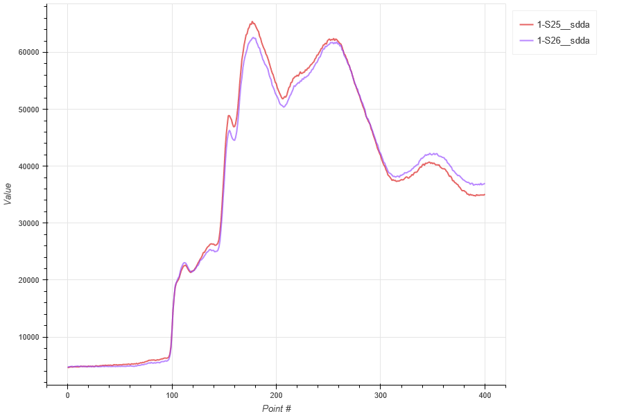
# Loading a series of scans
Simple = SimpleLoader()
Simple.load(RIXS,'HDF5_Notebook', 'sdda',25,26)
Simple.plot()
Simple.export('Simple_Data')
Python
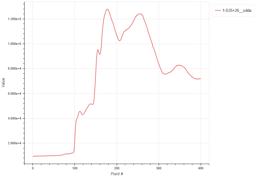
## Adding a series of scans
Plot = PlotLoader()
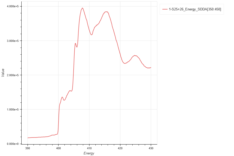
Plot.add(RIXS,'HDF5_Notebook', 'Energy', 'SDDA[350:450]',25,26)
Plot.plot()
Plot.export('Simple_Data')
PlotLoader()
Loads REIXS 1D or 1D Reduced Data
Class Information
Python
## PLOTING 1-D GENERAL DATA ##
Plot = PlotLoader()

## LOADING/ADDING/SUBSTRACTING 1-D/REDUCED DATA FROM A FILE ##
## Loads 1-D/Reduced scans data from HDF5 file
Plot.load(config,'filename', 'x_stream', 'y_stream', *args, **kwargs)
## *args = comma seperated list of scans to be plotted

## Loads and sums 1-D/Reduced scans data from HDF5 file
Plot.add(config,'filename', 'x_stream', 'y_stream', *args, **kwargs)
## *args = comma seperated list of scans to be plotted or added and then plotted

## Loads and subtracts 1-D/Reduced scans data from HDF5 file
Plot.subtract(config,'filename', 'x_stream', 'y_stream', *args, **kwargs)
## *args = s1, p1 -> The data from p1 is subtracted from s1
## *args = [s1, ..., sn], [p1, ..., pn] -> The sum of p1..pn is subtracted from the sum of s1...sn

## Loads and stitches 1-D/Reduced scans data from HDF5 file
Plot.stitch(config,'filename','x_stream', 'y_stream', *args, **kwargs)
## *args = comma seperated list of scans to be stitched

## Loads and subtract scan from all previously loaded scans
Plot.background(config,'filename', 'x_stream', 'y_stream', *args, **kwargs)
## *args = s1 -> The scan to be subtracted from all previous load/add/subtract actions
## *args = [s1, ..., sn] -> The sum of scans s1..sn to be subtracted from all previous load/add/subtract

## REQUIRED VARIABLES ##
## config = RIXS -> RIXS Endstation
## config = RSXS -> RSXS Endstation
## filename = hdf5 filename -> extenstion not required
## x_stream -> x-axis values, any mne or list from documentation
## y_stream -> y-axis values, any mne or list from documentation
## NOTE: Simple math allowed with xes_stream with contstants and variables, i.e. +, -, /, *

## NOTES ON X and Y STREAMS ##
## The total sum of dimensions of the x_stream and y_stream need to be 2
## For example, x_stream = 0 and y_stream = 2, or x_stream = 1 and y_stream = 1
## The axis reduction for 1-D data types is x_stream[min:max] reducing dimension to 0
## The axis reduction for 2-D data types is y_stream[min:max] reducing dimension to 1
## The axis reduction for 3-D data types is y_stream[{min:max}, None:None] reducing dimension to 2
## The axis reduction for 3-D data types is y_stream[{min1:max1}, {min2:max2}] reducing dimension to 1

## **kwargs ##
## norm = True -> Scales the data such that its range is 0 to 1.
## twin_y = True -> Adds these plots to a secondary scale
## xoffset = [(S1,P1),...,(SN,PN)] -> Adjusts x-axis scale to map SN to PN
## xcoffset = value -> Shifts x-axis scale by a constant value
## yoffset = [(S1,P1),...,(SN,PN)] -> Adjusts y-axis scale to map SN to PN
## ycoffset = value -> Shifts y-axis scale by a constant value
## grid = [start,stop,delta] -> Change x-axis grid to be uniform
## savgol = (length, poly ord, derv) -> Smooths and takes derivative
## binsize = bins -> Bins data, specify the number of points (extra points removed)

## SET RANGE OF X OR Y VALUES ##
Plot.xlim(min, max)
Plot.ylim(min, max)

# PLOTTING SCAN DATA ##
Plot.plot(**kwargs)

## **kwargs ##
## title = 'New Title of plot' -> Replaces default title with user defined
## xlabel = 'x-axis label' -> Replaces default x-axis label with user defined
## ylabel = 'y-axis label' -> Replaces default y-axis label with user defined
## ylabel_right = 'right y-axis label' -> Replaces default right y-axis label with user defined
## plot_height = value -> The plot height in points, default is 600
## plot_width = value -> The plot width in points, default is 900
## norm = True -> Normalizes all the data between 0 and 1
## waterfall = offset -> Normalizes as above and shifts each by the offset

## EXPORTING PLOT DATA ##
Plot.export('filename', **kwargs)

# REQUIRED VARIABLES ##
## filename = filename to be used for ASCII file, do not add extension
## NOTE: Data is exported as it displayed, only options in plotting methods are ignored.

## **kwargs ##
## split_files = True -> Saves each data stream with number appended to the filename
Examples
Python
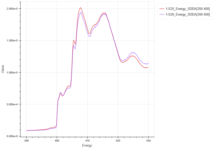
## Loading a series of scans
Plot = PlotLoader()
Plot.load(RIXS,'HDF5_Notebook', 'Energy', 'SDDA[350:450]',25,26)
Plot.plot()
Plot.export('Simple_Data')
Python
## Adding a series of scans
Plot = PlotLoader()
Plot.add(RIXS,'HDF5_Notebook', 'Energy', 'SDDA[350:450]',25,26)
Plot.plot()
Plot.export('Simple_Data')
ImageLoader()
Loads REIXS 2D or 2D Reduced Data
Class Information
Python
## PLOTING 2-D GENERAL DATA ##
Image = ImageLoader()

## LOADING/ADDING/SUBSTRACTING 2-D/REDUCED DATA FROM A FILE ##
## Loads 2-D/Reduced scans data from HDF5 file
Image.load(config,'filename', 'x_stream', 'detector', arg, **kwargs)
## args = scan number to be loaded

## Loads and sums 2-D/Reduced scans data from HDF5 file
Image.add(config,'filename', 'x_stream', 'detector', *args, **kwargs)
## *args = comma seperated list of scans to be plotted or added and then plotted

## Loads and subtracts 2-D/Reduced scans data from HDF5 file
Image.subtract(config,'filename', 'x_stream', 'detector', *args, **kwargs)
## *args = s1, p1 -> The data from p1 is subtracted from s1
## *args = [s1, ..., sn], [p1, ..., pn] -> The sum of p1..pn is subtracted from the sum of s1...sn

## Loads and stitches 2-D/Reduced scans data from HDF5 file
Image.stitch(config,'filename','x_stream', 'detector', *args, **kwargs)
## *args = comma seperated list of scans to be stitched

## Loads and subtracts the background from each image column
Image.background_1d(config,'filename','x_stream', 'detector', *args, **kwargs)
## *args = s1 -> The scan to be subtracted from all previous load/add/subtract actions
## *args = [s1, ..., sn] -> The sum of scans s1..sn to be subtracted from load/add/subtract

## Loads and subtracts the image the loaded image
Image.background_2d(config,'filename','x_stream', 'detector', *args, **kwargs)
## *args = s1 -> The scan to be subtracted from all previous load/add/subtract actions
## *args = [s1, ..., sn] -> The sum of scans s1..sn to be subtracted from load/add/subtract

## REQUIRED VARIABLES ##
## config = RIXS -> RIXS Endstation
## config = RSXS -> RSXS Endstation
## filename = hdf5 file -> Extension .h5 not needed
## x_stream -> x-axis values, any mne or list from documentation
## detector -> y-axis values, any mne or list from documentation
## NOTE: Simple math allowed with xes_stream with contstants and variables, i.e. +, -, /, *

## NOTES ON X STREAMS AND DETECTORS ##
## The total sum of dimensions of the x_stream and y_stream need to be 3
## For example, x_stream = 1 and y_stream = 2, or x_stream = 0 and y_stream = 3
## The axis reduction for 1-D data types is x_stream[min:max] reducing dimension to 0
## The axis reduction for 3-D data types is y_stream[{min:max}, None:None] reducing dimension to 2

## *kwargs options ##
## norm = True -> Scales the data such that its range is 0 to 1.
## xoffset = [(S1,P1),...,(SN,PN)] -> Adjusts x-axis scale to map SN to PN
## xcoffset = value -> Shifts x-axis scale by a constant value
## yoffset = [(S1,P1),...,(SN,PN)] -> Adjusts y-axis scale to map SN to PN
## ycoffset = value -> Shifts y-axis scale by a constant value
## grid_x = [start,stop,delta] -> Change x-axis grid to be uniform
## grid_y = [start,stop,delta] -> Change y-axis grid to be uniform
## binsize_x = bins -> Bins data along x-axis, specify the number of points (extra points removed)
## binsize_y = bins -> Bins data along y-axis, specify the number of points (extra points removed)

## SET RANGE OF Y and X VALUES ##
Image.xlim(min, max)
Image.ylim(min, max)

# PLOTTING SCAN DATA ##
Image.plot(**kwargs)

## **kwargs ##
## title = 'New Title of plot' -> Replaces default title with user defined
## xlabel = 'x-axis label' -> Replaces default x-axis label with user defined
## ylabel = 'y-axis label' -> Replaces default y-axis label with user defined
## zlabel = 'colorscale label' -> Replaces default colorscale label with user defined
## plot_height = value -> The plot height in points, default is 600
## plot_width = value -> The plot width in points, default is 900
## norm = True -> Normalizes all the data between 0 and 1
## vmin = value -> Sets the maximum value of the colorscale
## vmax = value -> Sets the minimum value of the colorscale

## EXPORTING PLOT DATA ##
Image.export('filename', **kwargs)

# REQUIRED VARIABLES ##
## filename = filename to be used for ASCII file, do not add extension
## NOTE: Data is exported as it displayed, only options in plotting methods are ignored.

## **kwargs ##
## split_files = True -> Saves each data stream with number appended to the filename
Examples
Python
## Loading a single scan
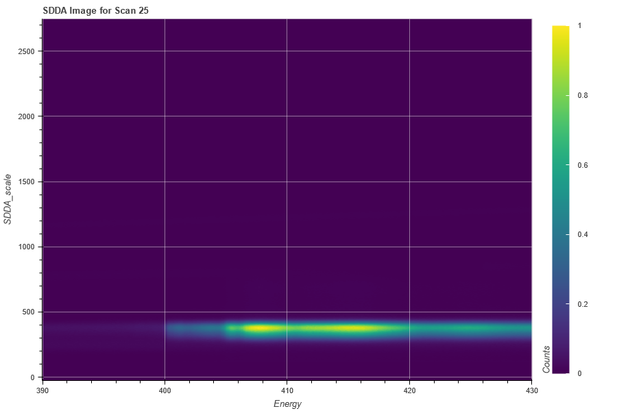
Image = ImageLoader()
Image.load(RIXS,'HDF5_Notebook', 'Energy', 'SDDA',25)
Image.plot(norm=True)
Image.export('Image_Load', split_files = True)
Python
## Adding a series of scans
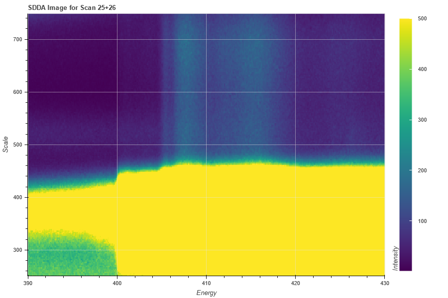
Image = ImageLoader()
Image.add(RIXS,'HDF5_Notebook', 'Energy', 'SDDA',25,26)
Image.ylim(250,750)
Image.plot(vmax = 500, zlabel = 'Intensity')
Image.export('Image_Add')
MeshLoader()
Loads REIXS Mesh Data
Class Information
Python
## PLOTING MESH DATA ##
Mesh = MESHLoader()

## LOADING/ADDING/SUBSTRACTING 2-D/REDUCED DATA FROM A FILE ##
## Loads 2-D/Reduced scans data from HDF5 file
Mesh.load(config,'filename', 'x_stream', 'y_stream', 'z_stream', arg, **kwargs)
## args = scan number to be loaded

## Loads and sums 2-D/Reduced scans data from HDF5 file
Mesh.add(config,'filename', 'x_stream', 'y_stream', 'z_stream', arg, **kwargs)
## *args = comma seperated list of scans to be plotted or added and then plotted

## Loads and subtracts 2-D/Reduced scans data from HDF5 file
Mesh.subtract(config,'filename', 'x_stream', 'y_stream', 'z_stream', arg, **kwargs)
## *args = s1, p1 -> The data from p1 is subtracted from s1
## *args = [s1, ..., sn], [p1, ..., pn] -> The sum of p1..pn is subtracted from the sum of s1...sn

## Loads and stitches 2-D/Reduced scans data from HDF5 file
Mesh.stitch(config,'filename','x_stream', 'y_stream', 'z_stream', arg, **kwargs)'
## *args = comma seperated list of scans to be stitched

## REQUIRED VARIABLES ##
## config = RIXS -> RIXS Endstation
## config = RSXS -> RSXS Endstation
## filename = hdf5 file -> Extension .h5 not needed
## x_stream -> x-axis values, any mne or list from documentation
## y_stream -> y-axis values, any mne or list from documentation
## z_stream -> z-axis values, any mne or list from documentation
## NOTE: Simple math allowed with xes_stream with contstants and variables, i.e. +, -, /, *

## NOTES ON X,Y,Z STREAMS ##
## The total sum of dimensions of the x_stream and y_stream need to be 3
## All streams need to have dimension 1

## *kwargs options ##
## norm = True -> Scales the data such that its range is 0 to 1.
## xoffset = [(S1,P1),...,(SN,PN)] -> Adjusts x-axis scale to map SN to PN
## xcoffset = value -> Shifts x-axis scale by a constant value
## yoffset = [(S1,P1),...,(SN,PN)] -> Adjusts y-axis scale to map SN to PN
## ycoffset = value -> Shifts y-axis scale by a constant value
## binsize_x = bins -> Bins data along x-axis, specify the number of points (extra points removed)
## binsize_y = bins -> Bins data along y-axis, specify the number of points (extra points removed)

## SET RANGE OF Y and X VALUES ##
Mesh.xlim(min, max)
Mesh.ylim(min, max)

# PLOTTING SCAN DATA ##
Mesh.plot(**kwargs)

## **kwargs ##
## title = 'New Title of plot' -> Replaces default title with user defined
## xlabel = 'x-axis label' -> Replaces default x-axis label with user defined
## ylabel = 'y-axis label' -> Replaces default y-axis label with user defined
## zlabel = 'colorscale label' -> Replaces default colorscale label with user defined
## plot_height = value -> The plot height in points, default is 600
## plot_width = value -> The plot width in points, default is 900
## norm = True -> Normalizes all the data between 0 and 1
## vmin = value -> Sets the maximum value of the colorscale
## vmax = value -> Sets the minimum value of the colorscale

## EXPORTING PLOT DATA ##
Mesh.export('filename', **kwargs)

# REQUIRED VARIABLES ##
## filename = filename to be used for ASCII file, do not add extension
## NOTE: Data is exported as it displayed, only options in plotting methods are ignored.

## **kwargs ##
## split_files = True -> Saves each data stream with number appended to the filename
Examples
Python
## Loading Raster Mesh scan
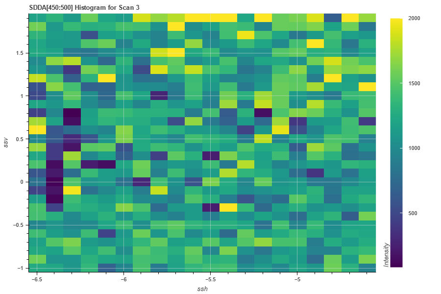
Mesh = MeshLoader()
Mesh.load(RIXS, 'HDF5_Notebook', 'ssh', 'ssv' ,'SDDA[450:500]', 3)
Mesh.xlim(-6.5, -4.5)
Mesh.ylim(-1,2)
Mesh.plot(vmax=2000,zlabel = 'Intensity')
Mesh.export('Mesh_Test')
StackLoader()
Loads REIXS 3D Image Stack
Class Information
Python
## PLOTING 3-D GENERAL DATA ##
Stack = StackLoader()

## LOADING/ADDING/SUBSTRACTING 3-D DATA FROM A FILE ##
## Loads 3-D scans data from HDF5 file
Stack.load(config,'filename', 'scan_stream', 'detector', arg, **kwargs)
## args = scan number to be loaded

## Loads and sums 3-D scans data from HDF5 file
Stack.add(config,'filename', 'scan_stream', 'detector', *args, **kwargs)
## *args = comma seperated list of scans to be plotted or added and then plotted

## Loads and subtracts 3-D scans data from HDF5 file
Stack.subtract(config,'filename', 'scan_stream', 'detector', *args, **kwargs)
## *args = s1, p1 -> The data from p1 is subtracted from s1
## *args = [s1, ..., sn], [p1, ..., pn] -> The sum of p1..pn is subtracted from the sum of s1...sn

## REQUIRED VARIABLES ##
## config = RIXS -> RIXS Endstation
## config = RSXS -> RSXS Endstation
## filename = hdf5 file -> Extension .h5 not needed
## scan_stream -> index values, any mne or list from documentation
## detector -> alias to image stream, needs to be stack of images
## NOTE: Simple math allowed with xes_stream with contstants and variables, i.e. +, -, /, *

## *kwargs options ##
## norm = True -> Scales the data such that its range is 0 to 1.
## xoffset = [(S1,P1),...,(SN,PN)] -> Adjusts x-axis scale to map SN to PN
## xcoffset = value -> Shifts x-axis scale by a constant value
## yoffset = [(S1,P1),...,(SN,PN)] -> Adjusts y-axis scale to map SN to PN
## ycoffset = value -> Shifts y-axis scale by a constant value
## grid_x = [start,stop,delta] -> Change x-axis grid to be uniform
## grid_y = [start,stop,delta] -> Change y-axis grid to be uniform

# PLOTTING SCAN DATA ##
Stack.plot(**kwargs)

## **kwargs ##
## title = 'New Title of plot' -> Replaces default title with user defined
## xlabel = 'x-axis label' -> Replaces default x-axis label with user defined
## ylabel = 'y-axis label' -> Replaces default y-axis label with user defined
## plot_height = value -> The plot height in points, default is 600
## plot_width = value -> The plot width in points, default is 900
## norm = True -> Normalizes all the data between 0 and 1

## EXPORTING PLOT DATA ##
Stack.export('filename', **kwargs)

# REQUIRED VARIABLES ##
## filename = filename to be used for ASCII file, do not add extension
## NOTE: Data is exported as it displayed, only options in plotting methods are ignored.

## **kwargs ##
## split_files = True -> Saves each data stream with number appended to the filename

## EXPORTING TO MOVIE ##
Stack.movie('filename', **kwargs)

# REQUIRED VARIABLES ##
## filename = filename to be used for mpeg file, do not add extension
## NOTE: Data is exported as it displayed, only options in plotting methods are ignored.

## **kwargs ##
## interval = value -> Duration of each frame ms
## aspect = fraction -> Ratio of vertical over horizontal
## xlim = (min, max) -> Sets the x-range of movie exported
## ylim = (min, max) -> Sets the y-range of movie exported
Examples
Python
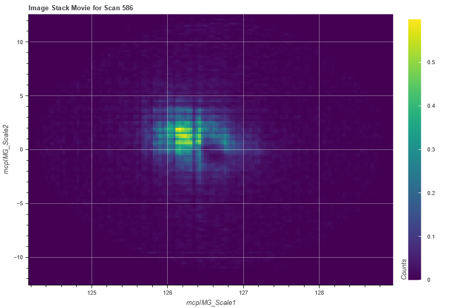
## Example of plotting stack
Stack = StackLoader()
Stack.load(RSXS, 'LNSCO110b', 'epoch','mcpIMG',586)
Stack.plot(norm = True)
Stack.movie('Movie_Scale', aspect = 0.25, xlim = (122,133), interval = 100)
Stack.export('Movie_ASCII')