PFYLoader()
Loads XAS Spectra with Complex ROIs
Class Information
Python
## PLOTING COMPLEX X-RAY ABSORPTION DATA ##
## Create an object named PFY to load XAS data with polygon ROI shape
PFY = PFYLoader()

## LOADING/ADDING/SUBSTRACTING 1-D/REDUCED DATA FROM A FILE ##
## Loads XES scans data from HDF5 file
PFY.load(config,'filename', 'detector', *args, **kwargs)
## *args = comma seperated list of scans to be plotted or added and then plotted

## Loads and sums XES scans data from HDF5 file
PFY.add(config,'filename', 'detector', *args, **kwargs)
## *args = comma seperated list of scans to be plotted or added and then plotted

## Loads and subtratcs XES scans data from HDF5 file
PFY.subtract(config,'filename', 'detector', *args, **kwargs)
## *args = s1, p1 -> The data from p1 is subtracted from s1
## *args = [s1, ..., sn], [p1, ..., pn] -> The sum of p1..pn is sub. from the sum s1...sn

## Loads and stitches non-overlapping regions
PFY.stitch(config,'filename', 'detector', *args, **kwargs)
## *args = comma seperated list of scans to be stitched
## NOTE: The the scans are appended in order, overlap discared

## Loads and subtract scan from all previously loaded scans
PFY.background(config,'filename', 'detector', *args, **kwargs)
## *args = s1 -> The scan to be subtracted from all previous load/add/subtract actions
## *args = [s1, ..., sn] -> The sum of scans s1..sn to be subtracted from load/add/subtract actions

## REQUIRED VARIABLES ##
## config = RIXS -> RIXS Endstation
## config = RSXS -> RSXS Endstation
## filename = hdf5 file -> Extension .h5 not needed
## detector -> sum of MCA type detector
## detector[Start:End] -> sums all MCA data within emission energy range
## detector[S1:E1,S2,E2] -> sums all MCA data within energy range S1 to E1 (start) and S2 to E2 (end)
## NOTE: Simple math allowed with xes_stream with contstants and variables, i.e. +, -, /, *

## **kwargs ##
## norm = True -> Scales the data such that its range is 0 to 1.
## twin_y = True -> Adds these plots to a secondary scale
## xoffset = [(S1,P1),...,(SN,PN)] -> Adjusts x-axis scale to map SN to PN
## xcoffset = value -> Shifts x-axis scale by a constant value
## yoffset = [(S1,P1),...,(SN,PN)] -> Adjusts y-axis scale to map SN to PN
## ycoffset = value -> Shifts y-axis scale by a constant value
## grid = [start,stop,delta] -> Change x-axis grid to be uniform
## savgol = (wind len, poly ord, derv) -> Smooths and takes derivative

## SET RANGE OF Y and X VALUES ##
PFY.xlim(min, max)
PFY.ylim(min, max)
## NOTE: These ranges will be preserved in the data export

## PLOTTING SCAN DATA ##
PFY.plot(**kwargs)

## **kwargs ##
## title = 'New Title of plot' -> Replaces default title with user defined
## xlabel = 'x-axis label' -> Replaces default x-axis label with user defined
## ylabel = 'y-axis label' -> Replaces default y-axis label with user defined
## plot_height = value -> The plot height in points, default is 600
## plot_width = value -> The plot width in points, default is 900
## norm = True -> Normalizes all the data between 0 and 1
## waterfall = offset -> Normalizes as above and shifts each by the offset

## EXPORTING PLOT DATA ##
PFY.export('filename', **kwargs)

## REQUIRED VARIABLES ##
## filename = filename to be used for ASCII file, do not add extension
## NOTE: Data is exported as it displayed, only options in plotting methods are ignored.

## **kwargs ##
## split_files = True -> Saves each data stream with number appended to the filename
Examples
Python
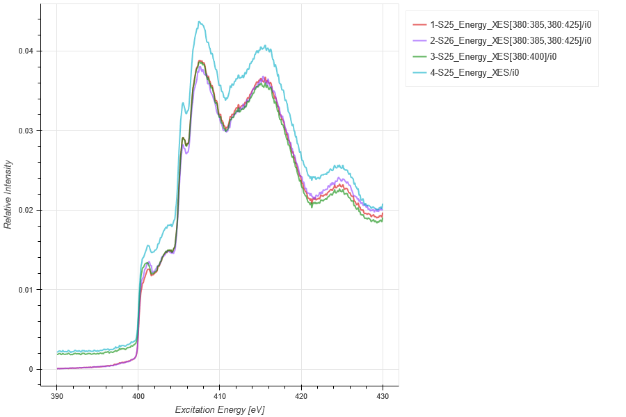
## Loading PFY data to remove elastic scattering and compare
PFY = PFYLoader()
PFY.load(RIXS, 'HDF5_Notebook', 'XES[380:385,380:425]/i0',25,26)
PFY.load(RIXS, 'HDF5_Notebook', 'XES[380:400]/i0',25)
PFY.load(RIXS, 'HDF5_Notebook', 'XES/i0',25)
PFY.plot()
PFY.export('PFY_Test')
ELOSSLoader()
Loads XES Spectra on Energy Loss Scale
Class Information
Python
## PLOTING XES DATA ON ENERGY LOSS SCALE ##
## Creates an object named XES to load XES DATA, EITHER TOTAL OR SUMMED OVER SPECIFIC ENERGIES
ELOSS = ELOSSLoader()

## LOADING/ADDING/SUBSTRACTING 1-D/REDUCED DATA FROM A FILE ##
## Loads XES scans data from HDF5 file
ELOSS.load(config,'filename', 'detector', *args, **kwargs)
## *args = comma seperated list of scans to be plotted or added and then plotted

## Loads and sums XES scans data from HDF5 file
ELOSS.add(config,'filename', 'detector', *args, **kwargs)
## *args = comma seperated list of scans to be plotted or added and then plotted

## Loads and subtratcs XES scans data from HDF5 file
ELOSS.subtract(config,'filename', 'detector', *args, **kwargs)
## *args = s1, p1 -> The data from p1 is subtracted from s1
## *args = [s1, ..., sn], [p1, ..., pn] -> The sum of p1..pn is sub. from the sum s1...sn

## Loads and stitches non-overlapping regions
ELOSS.stitch(config,'filename', 'detector', *args, **kwargs)
## *args = comma seperated list of scans to be stitched
## NOTE: The the scans are appended in order, overlap discared

## Loads and subtract scan from all previously loaded scans
ELOSS.background(config,'filename', 'detector', *args, **kwargs)
## *args = s1 -> The scan to be subtracted from all previous load/add/subtract actions
## *args = [s1, ..., sn] -> The sum of scans s1..sn to be subtracted from load/add/subtract actions

## REQUIRED VARIABLES ##
## config = RIXS -> RIXS Endstation
## config = RSXS -> RSXS Endstation
## filename = hdf5 file -> Extension .h5 not needed
## detector -> sums all data from MCA type detector
## detector[Start:End] -> sums all MCA data within excitation energy range
## NOTE: Simple math allowed with xes_stream with contstants and variables, i.e. +, -, /, *

## **kwargs ##
## norm = True -> Scales the data such that its range is 0 to 1.
## twin_y = True -> Adds these plots to a secondary scale
## xoffset = [(S1,P1),...,(SN,PN)] -> Adjusts x-axis scale to map SN to PN
## xcoffset = value -> Shifts x-axis scale by a constant value
## yoffset = [(S1,P1),...,(SN,PN)] -> Adjusts y-axis scale to map SN to PN
## ycoffset = value -> Shifts y-axis scale by a constant value
## grid = [start,stop,delta] -> Change x-axis grid to be uniform
## savgol = (wind len, poly ord, derv) -> Smooths and takes derivative
## binsize = bins -> Bins data bitwise, needs to be 2^N

## SET RANGE OF Y and X VALUES ##
ELOSS.xlim(min, max)
ELOSS.ylim(min, max)
## NOTE: These ranges will be preserved in the data export

## PLOTTING SCAN DATA ##
ELOSS.plot(**kwargs)

## **kwargs ##
## title = 'New Title of plot' -> Replaces default title with user defined
## xlabel = 'x-axis label' -> Replaces default x-axis label with user defined
## ylabel = 'y-axis label' -> Replaces default y-axis label with user defined
## plot_height = value -> The plot height in points, default is 600
## plot_width = value -> The plot width in points, default is 900
## norm = True -> Normalizes all the data between 0 and 1
## waterfall = offset -> Normalizes as above and shifts each by the offset

## EXPORTING PLOT DATA ##
ELOSS.export('filename', **kwargs)

## REQUIRED VARIABLES ##
## filename = filename to be used for ASCII file, do not add extension
## NOTE: Data is exported as it displayed, only options in plotting methods are ignored.

## **kwargs ##
## split_files = True -> Saves each data stream with number appended to the filename
Examples
Python
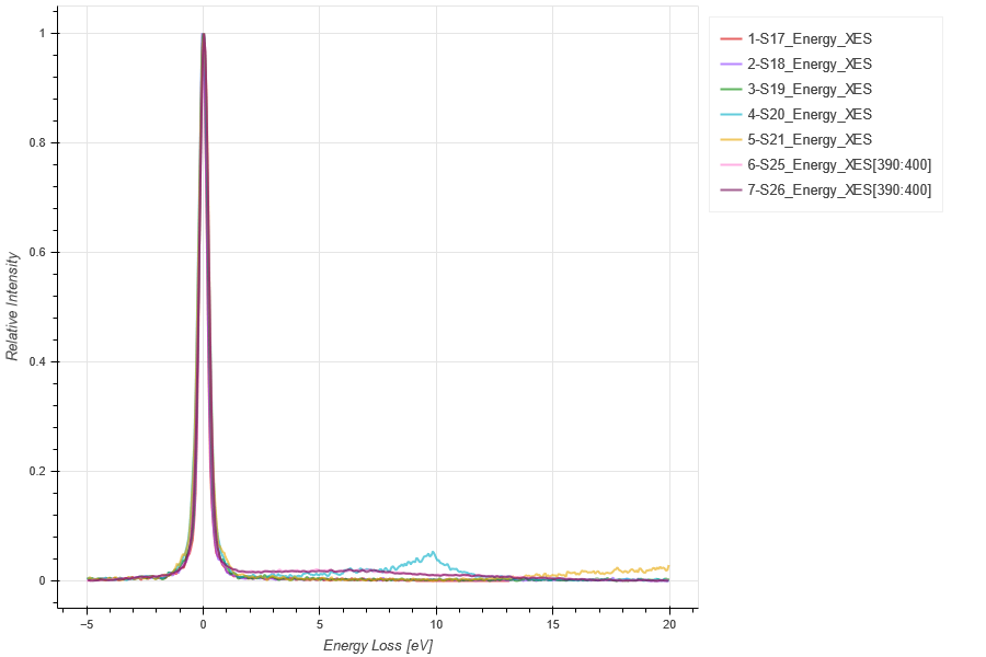
## Load various resonant hBN and Elastic Scatter Spectra
ELOSS = ELOSSLoader()
yoffset = [(369.438, 370), (379.393, 380), (389.210, 390), (398.932,400)]
ELOSS.load(RIXS,'HDF5_Notebook', 'XES', 17,18,19,20,21, yoffset = yoffset)
ELOSS.load(RIXS,'HDF5_Notebook', 'XES[390:400]', 25,26, yoffset = yoffset)
ELOSS.xlim(-5, 20)
ELOSS.plot(norm = True)
ELOSS.export('ELOSS1')
ELOSSMapper()
Loads XES/XAS Map with Energy Loss Scale
Class Information
Python
## PLOTING XES MAPS ON ENERGY LOSS SCALE ##
ELOSSMap = ELOSSMapper()

## LOADING/ADDING/SUBSTRACTING 2-D XES DATA FROM A FILE ##
## Loads 2-D XES scans data from HDF5 file
ELOSSMap.load(config,'filename', 'detector', arg, **kwargs)
## args = scan number to be loaded

## Loads and sums 2-D XES scans data from HDF5 file
ELOSSMap.add(config,'filename', 'detector', *args, **kwargs)
## *args = comma seperated list of scans to be plotted or added and then plotted

## Loads and subtracts 2-D XES scans data from HDF5 file
ELOSSMap.subtract(config,'filename', 'detector', *args, **kwargs)
## *args = s1, p1 -> The data from p1 is subtracted from s1
## *args = [s1, ..., sn], [p1, ..., pn] -> The sum of p1..pn is subtracted from the sum of s1...sn

## Loads and stitches 2-D XES scans data from HDF5 file
ELOSSMap.stitch(config,'filename','detector', *args, **kwargs)
## *args = comma seperated list of scans to be stitched

## Loads and subtracts the background from each image column
ELOSSMap.background_1d(config,'filename','detector', *args, **kwargs)
## *args = s1 -> The scan to be subtracted from all previous load/add/subtract actions
## *args = [s1, ..., sn] -> The sum of scans s1..sn to be subtracted from load/add/subtract

## Loads and subtracts the image the loaded image
ELOSSMap.background_2d(config,'filename','detector', *args, **kwargs)
## *args = s1 -> The scan to be subtracted from all previous load/add/subtract actions
## *args = [s1, ..., sn] -> The sum of scans s1..sn to be subtracted from load/add/subtract

## REQUIRED VARIABLES ##
## config = RIXS -> RIXS Endstation
## config = RSXS -> RSXS Endstation
## filename = hdf5 file -> Extension .h5 not needed
## xes_stream -> MCA type detector
## NOTE: Simple math allowed with xes_stream with contstants and variables, i.e. +, -, /, *

## *kwargs options ##
## norm = True -> Scales the data such that its range is 0 to 1.
## xoffset = [(S1,P1),...,(SN,PN)] -> Adjusts x-axis scale to map SN to PN
## xcoffset = value -> Shifts x-axis scale by a constant value
## yoffset = [(S1,P1),...,(SN,PN)] -> Adjusts y-axis scale to map SN to PN
## ycoffset = value -> Shifts y-axis scale by a constant value
## grid_x = [start,stop,delta] -> Change x-axis grid to be uniform
## grid_y = [start,stop,delta] -> Change y-axis grid to be uniform
## binsize_x = bins -> Bins data along x-axis, specify the number of points (extra points removed)
## binsize_y = bins -> Bins data along y-axis, specify the number of points (extra points removed)

## SET RANGE OF Y and X VALUES ##
ELOSSMap.xlim(min, max)
ELOSSMap.ylim(min, max)

# PLOTTING SCAN DATA ##
ELOSSMap.plot(**kwargs)

## **kwargs ##
## title = 'New Title of plot' -> Replaces default title with user defined
## xlabel = 'x-axis label' -> Replaces default x-axis label with user defined
## ylabel = 'y-axis label' -> Replaces default y-axis label with user defined
## zlabel = 'colorscale label' -> Replaces default colorscale label with user defined
## plot_height = value -> The plot height in points, default is 600
## plot_width = value -> The plot width in points, default is 900
## norm = True -> Normalizes all the data between 0 and 1
## vmin = value -> Sets the maximum value of the colorscale
## vmax = value -> Sets the minimum value of the colorscale

## EXPORTING PLOT DATA ##
ELOSSMap.export('filename', **kwargs)

# REQUIRED VARIABLES ##
## filename = filename to be used for ASCII file, do not add extension
## NOTE: Data is exported as it displayed, only options in plotting methods are ignored.

## **kwargs ##
## split_files = True -> Saves each data stream with number appended to the filename
Examples
Python
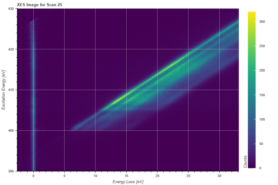
## ELOSS Map of hBN
ELOSSMap = ELOSSMapper()
yoffset = [(369.438, 370), (379.375, 380), (389.210, 390), (398.932, 400),(408.719, 410), (418.632, 420)]
ELOSSMap.load(RIXS, 'HDF5_Notebook' , 'XES', 25,yoffset = yoffset)
ELOSSMap.plot()
ELOSSMap.export('ELOSS_Map')