XESLoader()
Loads XES Spectra with Simple ROIs
Class Information
Python
## PLOTING X-RAY EMISSION SPECTROSCOPY DATA ##
## Creates an object named XES to load XES DATA, EITHER TOTAL OR SUMMED OVER SPECIFIC ENERGIES
XES = XESLoader()

## LOADING/ADDING/SUBSTRACTING 1-D/REDUCED DATA FROM A FILE ##
## Loads XES scans data from HDF5 file
XES.load(config,'filename', 'detector', *args, **kwargs)
## *args = comma seperated list of scans to be plotted or added and then plotted

## Loads and sums XES scans data from HDF5 file
XES.add(config,'filename', 'detector', *args, **kwargs)
## *args = comma seperated list of scans to be plotted or added and then plotted

## Loads and subtratcs XES scans data from HDF5 file
XES.subtract(config,'filename', 'detector', *args, **kwargs)
## *args = s1, p1 -> The data from p1 is subtracted from s1
## *args = [s1, ..., sn], [p1, ..., pn] -> The sum of p1..pn is sub. from the sum s1...sn

## Loads and stitches non-overlapping regions
XES.stitch(config,'filename', 'detector', *args, **kwargs)
## *args = comma seperated list of scans to be stitched
## NOTE: The the scans are appended in order, overlap discared

## Loads and subtract scan from all previously loaded scans
XES.background(config,'filename', 'detector', *args, **kwargs)
## *args = s1 -> The scan to be subtracted from all previous load/add/subtract actions
## *args = [s1, ..., sn] -> The sum of scans s1..sn to be subtracted from load/add/subtract actions

## REQUIRED VARIABLES ##
## config = RIXS -> RIXS Endstation
## config = RSXS -> RSXS Endstation
## filename = hdf5 file -> Extension .h5 not needed
## detector -> sums all data from MCA type detector
## detector[Start:End] -> sums all MCA data within excitation energy range
## NOTE: Simple math allowed with xes_stream with contstants and variables, i.e. +, -, /, *

## **kwargs ##
## norm = True -> Scales the data such that its range is 0 to 1.
## twin_y = True -> Adds these plots to a secondary scale
## xoffset = [(S1,P1),...,(SN,PN)] -> Adjusts x-axis scale to map SN to PN
## xcoffset = value -> Shifts x-axis scale by a constant value
## yoffset = [(S1,P1),...,(SN,PN)] -> Adjusts y-axis scale to map SN to PN
## ycoffset = value -> Shifts y-axis scale by a constant value
## grid = [start,stop,delta] -> Change x-axis grid to be uniform
## savgol = (wind len, poly ord, derv) -> Smooths and takes derivative
## binsize = bins -> Bins data, specify the number of points (extra points removed)

## SET RANGE OF Y and X VALUES ##
XES.xlim(min, max)
XES.ylim(min, max)
## NOTE: These ranges will be preserved in the data export

## PLOTTING SCAN DATA ##
XES.plot(**kwargs)

## **kwargs ##
## title = 'New Title of plot' -> Replaces default title with user defined
## xlabel = 'x-axis label' -> Replaces default x-axis label with user defined
## ylabel = 'y-axis label' -> Replaces default y-axis label with user defined
## plot_height = value -> The plot height in points, default is 600
## plot_width = value -> The plot width in points, default is 900
## norm = True -> Normalizes all the data between 0 and 1
## waterfall = offset -> Normalizes as above and shifts each by the offset

## EXPORTING PLOT DATA ##
XES.export('filename', **kwargs)

## REQUIRED VARIABLES ##
## filename = filename to be used for ASCII file, do not add extension
## NOTE: Data is exported as it displayed, only options in plotting methods are ignored.

## **kwargs ##
## split_files = True -> Saves each data stream with number appended to the filename
Examples
Python
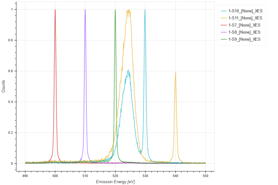
## Plot elastic peaks for calibration
## Add offset for scale mapping, apply to all subsequent scans
XES_Calib = XESLoader()
xoffset = [(498.442, 500), (508.254, 510), (517.910, 520), (527.574, 530),(537.059, 540)]
XES_Calib.load(RIXS,'HDF5_Notebook.h5','XES',7,8,9,10,11,xoffset= xoffset)
XES_Calib.xlim(490,550)
XES_Calib.plot(norm = True)
XES_Calib.export('XES_Calib')
Python
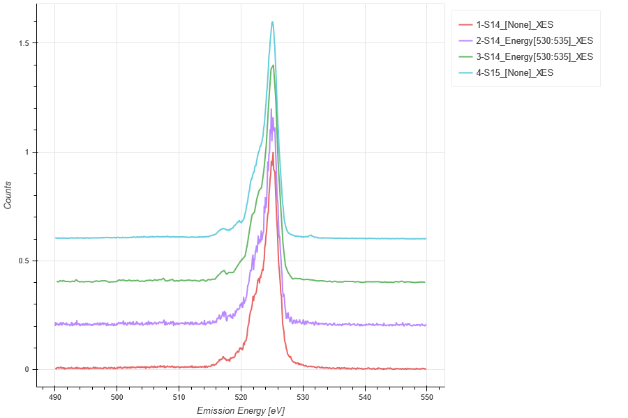
## Sum specific excitation energies of the scan and compare
## Bin the data to improve statisitcs
BGO_XES = XESLoader()
xoffset = [(498.442, 500), (508.254, 510), (517.910, 520), (527.574, 530),(537.059, 540)]
BGO_XES.load(RIXS,'HDF5_Notebook.h5','XES',14,xoffset = xoffset)
BGO_XES.load(RIXS,'HDF5_Notebook.h5','XES[530:535]',14,xoffset = xoffset)
BGO_XES.load(RIXS,'HDF5_Notebook.h5','XES[530:535]',14,binsize = 4,xoffset = xoffset)
BGO_XES.load(RIXS,'HDF5_Notebook.h5','XES',15,xoffset = xoffset)
BGO_XES.xlim(490,550)
BGO_XES.plot(waterfall = 0.2)
BGO_XES.export('BGO_XES')
XASLoader()
Loads XAS Spectra with Simple ROIs
Class Information
Python
## PLOTING X-RAY ABSORPTION SPECTROSCOPY DATA ##
## Creates an object named XAS to load XAS DATA, EITHER TOTAL OR SUMMED OVER SPECIFIC ENERGIES
XAS = XASLoader()

## LOADING/ADDING/SUBSTRACTING 1-D/REDUCED DATA FROM A FILE ##
## Loads XES scans data from HDF5 file
XAS.load(config,'filename', 'y_stream', *args, **kwargs)
## *args = comma seperated list of scans to be plotted or added and then plotted

## Loads and sums XES scans data from HDF5 file
XAS.add(config,'filename', 'y_stream', *args, **kwargs)
## *args = comma seperated list of scans to be plotted or added and then plotted

## Loads and subtratcs XES scans data from HDF5 file
XAS.subtract(config,'filename', 'y_stream', *args, **kwargs)
## *args = s1, p1 -> The data from p1 is subtracted from s1
## *args = [s1, ..., sn], [p1, ..., pn] -> The sum of p1..pn is sub. from the sum s1...sn

## Loads and stitches non-overlapping regions
XAS.stitch(config,'filename', 'xas_y_streamstream', *args, **kwargs)
## *args = comma seperated list of scans to be stitched
## NOTE: The the scans are appended in order, overlap discared

## Loads and subtract scan from all previously loaded scans
XAS.background(config,'filename', 'y_stream', *args, **kwargs)
## *args = s1 -> The scan to be subtracted from all previous load/add/subtract actions
## *args = [s1, ..., sn] -> The sum of scans s1..sn to be subtracted from load/add/subtract actions

## REQUIRED VARIABLES ##
## config = RIXS -> RIXS Endstation
## config = RSXS -> RSXS Endstation
## filename = hdf5 file -> Extension .h5 not needed
## y_stream -> SCA detector or sum of MCA type detector
## y_stream[Start:End] -> sums all MCA data within emission energy range
## y_stream[{S1:E1},{S2,E2}] -> ROI of image detector
## NOTE: Simple math allowed with xes_stream with contstants and variables, i.e. +, -, /, *

## **kwargs ##
## norm = True -> Scales the data such that its range is 0 to 1.
## twin_y = True -> Adds these plots to a secondary scale
## xoffset = [(S1,P1),...,(SN,PN)] -> Adjusts x-axis scale to map SN to PN
## xcoffset = value -> Shifts x-axis scale by a constant value
## yoffset = [(S1,P1),...,(SN,PN)] -> Adjusts y-axis scale to map SN to PN
## ycoffset = value -> Shifts y-axis scale by a constant value
## grid = [start,stop,delta] -> Change x-axis grid to be uniform
## savgol = (wind len, poly ord, derv) -> Smooths and takes derivative
## binsize = bins -> Bins data, specify the number of points (extra points removed)

## SET RANGE OF Y and X VALUES ##
XAS.xlim(min, max)
XAS.ylim(min, max)
## NOTE: These ranges will be preserved in the data export

## PLOTTING SCAN DATA ##
XAS.plot(**kwargs)

## **kwargs ##
## title = 'New Title of plot' -> Replaces default title with user defined
## xlabel = 'x-axis label' -> Replaces default x-axis label with user defined
## ylabel = 'y-axis label' -> Replaces default y-axis label with user defined
## plot_height = value -> The plot height in points, default is 600
## plot_width = value -> The plot width in points, default is 900
## norm = True -> Normalizes all the data between 0 and 1
## waterfall = offset -> Normalizes as above and shifts each by the offset

## EXPORTING PLOT DATA ##
XAS.export('filename', **kwargs)

## REQUIRED VARIABLES ##
## filename = filename to be used for ASCII file, do not add extension
## NOTE: Data is exported as it displayed, only options in plotting methods are ignored.

## **kwargs ##
## split_files = True -> Saves each data stream with number appended to the filename
Examples
Python
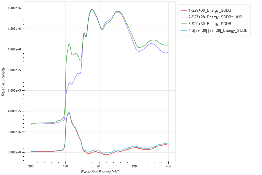
## Compare h-BN Polarization XAS
hBN_XAS = XASLoader()
hBN_XAS.add(RIXS,'HDF5_Notebook', 'SDDB',29,30)
hBN_XAS.background(RIXS,'HDF5_Notebook', 'SDDB*1.012',27,28)
hBN_XAS.add(RIXS,'HDF5_Notebook', 'SDDB*1.012',27,28)
hBN_XAS.add(RIXS,'HDF5_Notebook', 'SDDB',29,30)
hBN_XAS.subtract(RIXS,'HDF5_Notebook', 'SDDB',[29,30],[27,28])
hBN_XAS.plot()
hBN_XAS.export('hBN_XAS', split_files = True)
Python
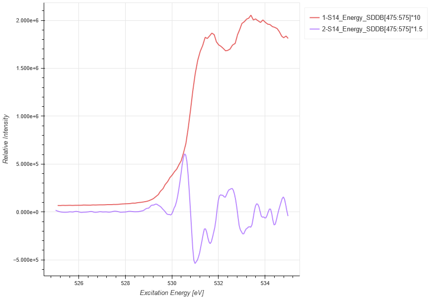
## BGO O 1s XAS, both with O Ka ROI and total
BGO_XAS = XASLoader()
BGO_XAS.load(RIXS,'HDF5_Notebook', 'SDDB[475:575]*10',14)
BGO_XAS.load(RIXS,'HDF5_Notebook', 'SDDB[475:575]*1.5',14, grid_x=(525,560, 0.05),savgol = (20,5,2))
BGO_XAS.xlim(525,535)
BGO_XAS.plot()
BGO_XAS.export('BGO_XAS')
XEOLLoader()
Loads XEOL Spectra with Simple ROIs
Class Information
Python
## PLOTING X-RAY EXCITED OPTICAL EMISSION DATA ##
## Creates an object named XEOL to load XEOL DATA, EITHER TOTAL OR SUMMED OVER SPECIFIC ENERGIES
XEOL = XEOLLoader()

## LOADING/ADDING/SUBSTRACTING XEOL DATA FROM A FILE ##
## Loads XEOL scans data from HDF5 file
XEOL.load(config,'filename', 'detector', *args, **kwargs)
## *args = comma seperated list of scans to be plotted or added and then plotted

## Loads and sums XES scans data from HDF5 file
XEOL.add(config,'filename', 'detector', *args, **kwargs)
## *args = comma seperated list of scans to be plotted or added and then plotted

## Loads and subtratcs XES scans data from HDF5 file
XEOL.subtract(config,'filename', 'detector', *args, **kwargs)
## *args = s1, p1 -> The data from p1 is subtracted from s1
## *args = [s1, ..., sn], [p1, ..., pn] -> The sum of p1..pn is sub. from the sum s1...sn

## Loads and subtract scan from all previously loaded scans
XEOL.background(config,'filename', 'detector', *args, **kwargs)
## *args = s1 -> The scan to be subtracted from all previous load/add/subtract actions
## *args = [s1, ..., sn] -> The sum of scans s1..sn to be subtracted from load/add/subtract actions

## REQUIRED VARIABLES ##
## config = RIXS -> RIXS Endstation
## config = RSXS -> RSXS Endstation
## filename = hdf5 file -> Extension .h5 not needed
## xeol_stream -> sums all data from MCA type detector
## xeol_stream[Start:End] -> sums all MCA data within excitation energy range
## NOTE: Simple math allowed with xes_stream with contstants and variables, i.e. +, -, /, *

## **kwargs ##
## norm = True -> Scales the data such that its range is 0 to 1.
## twin_y = True -> Adds these plots to a secondary scale
## xoffset = [(S1,P1),...,(SN,PN)] -> Adjusts x-axis scale to map SN to PN
## xcoffset = value -> Shifts x-axis scale by a constant value
## yoffset = [(S1,P1),...,(SN,PN)] -> Adjusts y-axis scale to map SN to PN
## ycoffset = value -> Shifts y-axis scale by a constant value
## grid = [start,stop,delta] -> Change x-axis grid to be uniform
## savgol = (wind len, poly ord, derv) -> Smooths and takes derivative
## binsize = bins -> Bins data, specify the number of points (extra points removed)

## SET RANGE OF Y and X VALUES ##
XEOL.xlim(min, max)
XEOL.ylim(min, max)
## NOTE: These ranges will be preserved in the data export

## PLOTTING SCAN DATA ##
XEOL.plot(**kwargs)

## **kwargs ##
## title = 'New Title of plot' -> Replaces default title with user defined
## xlabel = 'x-axis label' -> Replaces default x-axis label with user defined
## ylabel = 'y-axis label' -> Replaces default y-axis label with user defined
## plot_height = value -> The plot height in points, default is 600
## plot_width = value -> The plot width in points, default is 900
## norm = True -> Normalizes all the data between 0 and 1
## waterfall = offset -> Normalizes as above and shifts each by the offset

## EXPORTING PLOT DATA ##
XEOL.export('filename', **kwargs)

## REQUIRED VARIABLES ##
## filename = filename to be used for ASCII file, do not add extension
## NOTE: Data is exported as it displayed, only options in plotting methods are ignored.

## **kwargs ##
## split_files = True -> Saves each data stream with number appended to the filename
Examples
Python
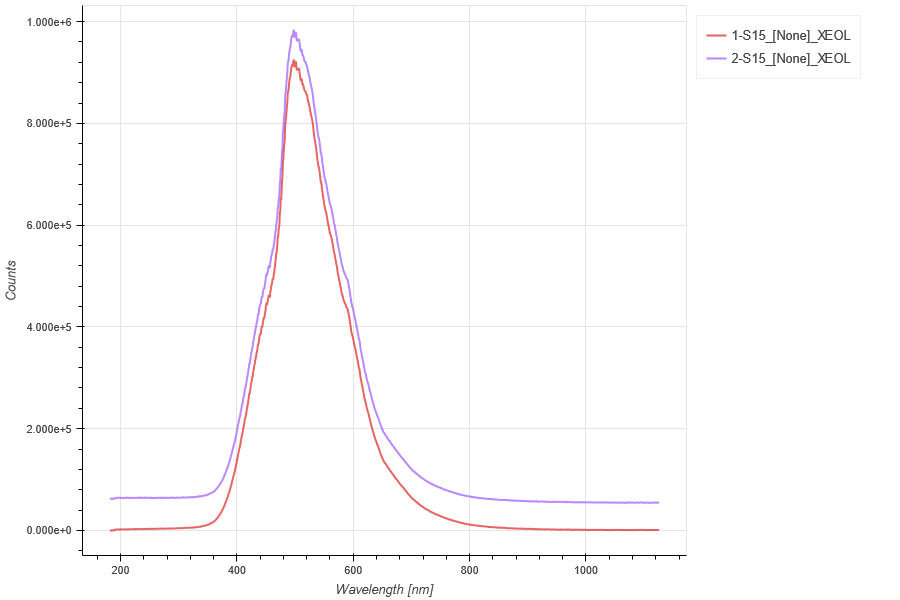
## XEOL Spectra from BGO
BGO_XEOL = XEOLLoader()
BGO_XEOL.load(RIXS, 'HDF5_Notebook', 'XEOL',15)
## Need to scale the background by exposures
BGO_XEOL.background(RIXS, 'HDF5_Notebook', 'XEOL/50*20', 16)
## Add in spectra with background substraction
BGO_XEOL.load(RIXS, 'HDF5_Notebook', 'XEOL',15)
BGO_XEOL.plot()
BGO_XEOL.export('BGO_XEOL')
Python
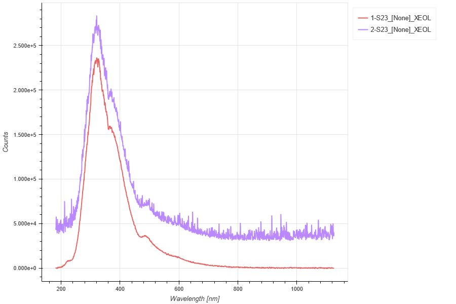
## XEOL Spectra from hBN
hBN_XEOL = XEOLLoader()
hBN_XEOL.load(RIXS, 'HDF5_Notebook', 'XEOL',23)
## Need to scale the background by exposures
hBN_XEOL.background(RIXS, 'HDF5_Notebook', 'XEOL/5*10', 24)
## Add in spectra with background substraction
hBN_XEOL.load(RIXS, 'HDF5_Notebook', 'XEOL',23)
hBN_XEOL.plot()
hBN_XEOL.export('hBN_XEOL')
XESMapper()
Loads XES/XAS Map
Class Information
Python
## PLOTING XES Maps ##
XESMap = XESMapper()

## LOADING/ADDING/SUBSTRACTING 2-D XES DATA FROM A FILE ##
## Loads 2-D XES scans data from HDF5 file
XESMap.load(config,'filename', 'detector', arg, **kwargs)
## args = scan number to be loaded

## Loads and sums 2-D XES scans data from HDF5 file
XESMap.add(config,'filename', 'detector', *args, **kwargs)
## *args = comma seperated list of scans to be plotted or added and then plotted

## Loads and subtracts 2-D XES scans data from HDF5 file
XESMap.subtract(config,'filename', 'detector', *args, **kwargs)
## *args = s1, p1 -> The data from p1 is subtracted from s1
## *args = [s1, ..., sn], [p1, ..., pn] -> The sum of p1..pn is subtracted from the sum of s1...sn

## Loads and stitches 2-D XES scans data from HDF5 file
XESMap.stitch(config,'filename','detector', *args, **kwargs)
## *args = comma seperated list of scans to be stitched

## Loads and subtracts the background from each image column
XESMap.background_1d(config,'filename','detector', *args, **kwargs)
## *args = s1 -> The scan to be subtracted from all previous load/add/subtract actions
## *args = [s1, ..., sn] -> The sum of scans s1..sn to be subtracted from load/add/subtract

## Loads and subtracts the image the loaded image
XESMap.background_2d(config,'filename','detector', *args, **kwargs)
## *args = s1 -> The scan to be subtracted from all previous load/add/subtract actions
## *args = [s1, ..., sn] -> The sum of scans s1..sn to be subtracted from load/add/subtract

## REQUIRED VARIABLES ##
## config = RIXS -> RIXS Endstation
## config = RSXS -> RSXS Endstation
## filename = hdf5 file -> Extension .h5 not needed
## detector -> MCA type detector
## NOTE: Simple math allowed with xes_stream with contstants and variables, i.e. +, -, /, *

## *kwargs options ##
## norm = True -> Scales the data such that its range is 0 to 1.
## xoffset = [(S1,P1),...,(SN,PN)] -> Adjusts x-axis scale to map SN to PN
## xcoffset = value -> Shifts x-axis scale by a constant value
## yoffset = [(S1,P1),...,(SN,PN)] -> Adjusts y-axis scale to map SN to PN
## ycoffset = value -> Shifts y-axis scale by a constant value
## grid_x = [start,stop,delta] -> Change x-axis grid to be uniform
## grid_y = [start,stop,delta] -> Change y-axis grid to be uniform
## binsize_x = bins -> Bins data along x-axis, specify the number of points (extra points removed)
## binsize_y = bins -> Bins data along y-axis, specify the number of points (extra points removed)

## SET RANGE OF Y and X VALUES ##
XESMap.xlim(min, max)
XESMap.ylim(min, max)

# PLOTTING SCAN DATA ##
XESMap.plot(**kwargs)

## **kwargs ##
## title = 'New Title of plot' -> Replaces default title with user defined
## xlabel = 'x-axis label' -> Replaces default x-axis label with user defined
## ylabel = 'y-axis label' -> Replaces default y-axis label with user defined
## zlabel = 'colorscale label' -> Replaces default colorscale label with user defined
## plot_height = value -> The plot height in points, default is 600
## plot_width = value -> The plot width in points, default is 900
## norm = True -> Normalizes all the data between 0 and 1
## vmin = value -> Sets the maximum value of the colorscale
## vmax = value -> Sets the minimum value of the colorscale

## EXPORTING PLOT DATA ##
XESMap.export('filename', **kwargs)

# REQUIRED VARIABLES ##
## filename = filename to be used for ASCII file, do not add extension
## NOTE: Data is exported as it displayed, only options in plotting methods are ignored.

## **kwargs ##
## split_files = True -> Saves each data stream with number appended to the filename
Examples
Python
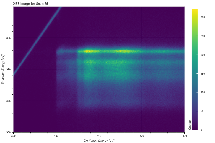
## Plot of XES Map
XESMap = XESMapper()
XESMap.load(RIXS, 'HDF5_Notebook' , 'XES', 25)
XESMap.ylim(380,400)
XESMap.plot()
XESMap.export('XES_Map')
XEOLMapper()
Loads XEOL/XAS Map
Class Information
Python
## PLOTING XEOL Maps ##
XEOLMap = XEOLMapper()

## LOADING/ADDING/SUBSTRACTING 2-D XEOL DATA FROM A FILE ##
## Loads 2-D XES scans data from HDF5 file
XEOLMap.load(config,'filename', 'detector', arg, **kwargs)
## args = scan number to be loaded

## Loads and sums 2-D XEOL scans data from HDF5 file
XEOLMap.add(config,'filename', 'detector', *args, **kwargs)
## *args = comma seperated list of scans to be plotted or added and then plotted

## Loads and subtracts 2-D XEOL scans data from HDF5 file
XEOLMap.subtract(config,'filename', 'detector', *args, **kwargs)
## *args = s1, p1 -> The data from p1 is subtracted from s1
## *args = [s1, ..., sn], [p1, ..., pn] -> The sum of p1..pn is subtracted from the sum of s1...sn

## Loads and stitches 2-D XEOL scans data from HDF5 file
XEOLMap.stitch(config,'filename','detector', *args, **kwargs)
## *args = comma seperated list of scans to be stitched

## Loads and subtracts the background from each image column
XEOLMap.background_1d(config,'filename','detector', *args, **kwargs)
## *args = s1 -> The scan to be subtracted from all previous load/add/subtract actions
## *args = [s1, ..., sn] -> The sum of scans s1..sn to be subtracted from load/add/subtract

## Loads and subtracts the image the loaded image
XEOLMap.background_2d(config,'filename','detector', *args, **kwargs)
## *args = s1 -> The scan to be subtracted from all previous load/add/subtract actions
## *args = [s1, ..., sn] -> The sum of scans s1..sn to be subtracted from load/add/subtract

## REQUIRED VARIABLES ##
## config = RIXS -> RIXS Endstation
## config = RSXS -> RSXS Endstation
## filename = hdf5 file -> Extension .h5 not needed
## detector -> MCA type detector
## NOTE: Simple math allowed with xes_stream with contstants and variables, i.e. +, -, /, *

## *kwargs options ##
## norm = True -> Scales the data such that its range is 0 to 1.
## xoffset = [(S1,P1),...,(SN,PN)] -> Adjusts x-axis scale to map SN to PN
## xcoffset = value -> Shifts x-axis scale by a constant value
## yoffset = [(S1,P1),...,(SN,PN)] -> Adjusts y-axis scale to map SN to PN
## ycoffset = value -> Shifts y-axis scale by a constant value
## grid_x = [start,stop,delta] -> Change x-axis grid to be uniform
## grid_y = [start,stop,delta] -> Change y-axis grid to be uniform
## binsize_x = bins -> Bins data along x-axis, specify the number of points (extra points removed)
## binsize_y = bins -> Bins data along y-axis, specify the number of points (extra points removed)

## SET RANGE OF Y and X VALUES ##
XEOLMap.xlim(min, max)
XEOLMap.ylim(min, max)

# PLOTTING SCAN DATA ##
XEOLMap.plot(**kwargs)

## **kwargs ##
## title = 'New Title of plot' -> Replaces default title with user defined
## xlabel = 'x-axis label' -> Replaces default x-axis label with user defined
## ylabel = 'y-axis label' -> Replaces default y-axis label with user defined
## zlabel = 'colorscale label' -> Replaces default colorscale label with user defined
## plot_height = value -> The plot height in points, default is 600
## plot_width = value -> The plot width in points, default is 900
## norm = True -> Normalizes all the data between 0 and 1
## vmin = value -> Sets the maximum value of the colorscale
## vmax = value -> Sets the minimum value of the colorscale

## EXPORTING PLOT DATA ##
XEOLMap.export('filename', **kwargs)

# REQUIRED VARIABLES ##
## filename = filename to be used for ASCII file, do not add extension
## NOTE: Data is exported as it displayed, only options in plotting methods are ignored.

## **kwargs ##
## split_files = True -> Saves each data stream with number appended to the filename
Examples
Python
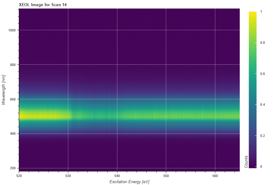
## XEOL Map with Background Subtracted
XEOLMap = XEOLMapper()
XEOLMap.load(RIXS, 'HDF5_Notebook', 'XEOL', 14)
XEOLMap.background_1d(RIXS, 'HDF5_Notebook','XEOL/50', 16)
XEOLMap.plot(norm = True)
XEOLMap.export('XEOL_Map')